From Fair Value Gaps to Brownian Motion — Building the Bridge

Introduction

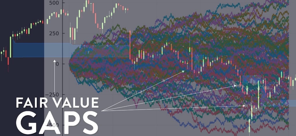
Traders using Fair Value Gaps (FVGs) often rely on price inefficiencies—imbalances in supply and demand—to anticipate mean reversion or continuation. While this is powerful in practice, a deeper edge comes from quantitative theory. Concepts like Brownian Motion and Stochastic Calculus form the basis of option pricing and volatility modeling—and unlock insights beyond pattern recognition.

This article begins a journey into the mathematical structure behind markets, making you not just a practitioner, but a master of probabilistic modeling and risk.

Brownian Motion: The Bedrock of Market Randomness

Brownian Motion (aka Wiener Process) is a mathematical model for randomness that satisfies:

1. Independent Increments: Price moves today are independent of past moves.

2. Stationary Increments: The change over a time interval only depends on the length of that interval.

3. Normal Distribution: Increments are normally distributed with zero mean and variance proportional to time.

4. Continuous Paths: No sudden jumps, unlike real markets—but a useful approximation.

Why This Matters for Traders

Every time you look at a candlestick chart, you're witnessing a noisy signal. Brownian Motion is a mathematical idealization of that noise. It’s the first step toward modeling volatility, options, and fair value under uncertainty.

Stochastic Calculus: The Language of Dynamic Risk

To model real-time price behavior, we need to move beyond classical calculus. Why?

Because in standard calculus:

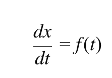
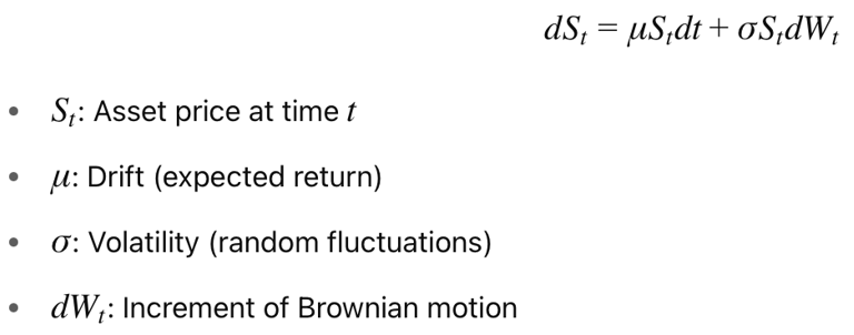
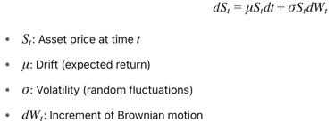
But if x(t) is a Brownian path, it's nowhere differentiable—too erratic. Enter Stochastic Calculus, and especially Itô Calculus, which allows us to define:

This is called Geometric Brownian Motion—a core model in Black-Scholes option pricing.

Volatility as Energy: A Physical Analogy

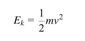
In physics, Kinetic Energy is:

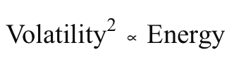
If you think of volatility as the speed of price movement, and assume “mass” as constant (e.g., 1), then:

This analogy is more than poetic—it motivates models like:

• GARCH (Generalized Autoregressive Conditional Heteroskedasticity): Volatility clusters like turbulent energy.

• Heston Model: Models volatility as a stochastic process, like the chaotic energy of particles.

This helps explain why price expands and contracts around FVG zones—energy builds and releases, creating imbalances and corrections.

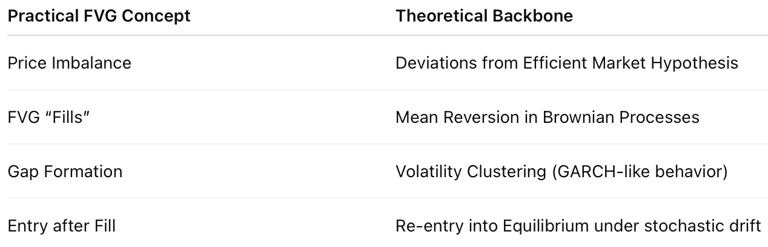
Connecting the Dots: FVG Meets Quant Models

Your trading edge using FVG can be enhanced by understanding:

Final Thoughts

By learning the language of randomness, you're not abandoning your edge in price action—you're strengthening it. Brownian Motion and Stochastic Calculus give you the tools to model uncertainty itself.

Stay tuned, and follow the path from intuition to equation.

References

1. Shreve, S. E. (2004). Stochastic Calculus for Finance I & II. Springer Finance.

2. Hull, J. C. (2015). Options, Futures, and Other Derivatives (9th ed.). Pearson.

3. Björk, T. (2009). Arbitrage Theory in Continuous Time. Oxford University Press.

4. Engle, R. (1982). "Autoregressive Conditional Heteroscedasticity with Estimates of the Variance of United Kingdom Inflation." Econometrica.

5. Black, F., & Scholes, M. (1973). "The Pricing of Options and Corporate Liabilities." Journal of Political Economy.

6. Heston, S. L. (1993). "A Closed-Form Solution for Options with Stochastic Volatility with Applications to Bond and Currency Options." The Review of Financial Studies.

7. Karatzas, I., & Shreve, S. E. (1991). Brownian Motion and Stochastic Calculus. Springer.

8. Gatheral, J. (2006). The Volatility Surface: A Practitioner's Guide. Wiley Finance.